Getting started with the VM

Find out the opencv.ova VM for this Workshop at ngcmbits (available soon) or an alternative way(the link is also available at Trello on the OpenCV tab). If you are using a new VM follow the next steps. On the other hand, if you have downloaded the provided machine jump to the Workshop material section to pull the latest changes in the repository.

$ sudo apt-get install update

After updating the sources of the repositories, it is time to install some dependencies, normally these ones should be available in a full Ubuntu version but as we are dealing with a minimal version it is required to do it manually.

$ sudo apt-get install gcc make

The next step is to install the Guest additions. As you probably have noticed the screen of your VM does not fit your real resolution, this is one of the main features that is going to solve the installation of the additions.

Go to the Virtual Box options, find the Devices tab and click Insert Guest Additions. After this step, open a terminal window and type the following command:

$ cd /media/feeg6003/VirtualBox...
$ sudo sh ./VBoxLinuxAdditions.run

Once the installation is completed you will be asked to restart your VM. Please do so and you will be able to fit the screen to the real resolution using the desktop preferences.

OpenCV - Python Installation

To perform the installation of the OpenCv library for python there are two ways to do it:

The first one is installing only the libraries for python using pre-built libraries typing the following commands:

$ sudo apt-get install python-opencv
$ sudo apt-get install python-numpy
$ sudo apt-get install python-matplotlib
$ sudo apt-get install ffmpeg

To check if everything it is been successfully installed open a Python IDLE and type the following commands:

import cv2
print cv2.__version__

If the version displayed is 3.1.0 or greater you are in good position to continue.

The second option, is to download the source code and compile the whole code. This is a long and tedious installation, so the recommendation is to do it with the previous commands.

Check “Building OpenCV from source” to follow the steps. Consult the OpenCV guide

Workshop material

Pulling last version of the repository examples

In order to get the samples to complete and the solutions from the workshop, the next command can be used to download all the sources from Bitbucket. Inside the repository you will be able to finde a folder named 'examples' where to can find all of this codes also and the images and videos used over this blog.

$ sudo apt-get install mercurial
$ cd $HOME
$ hg clone https://josemgf@bitbucket.org/josemgf/opencv-feeg6003
$ cd opencv-feeg6003
$ hg pull
$ hg update

The slides can be downloaded using the following link: slides.

OpenCV

OpenCV is an open source library used for image processing and machine learning. It was built to provide a common infrastructure for computer vision applications.

The library contains more than 2500 algorithms, from the basics of getting images and changing the color to the most complex algorithms to extract 3d objects from an image. Passing through removing the red eyes and tracking objects for example.

This is a cross-platform library having available interfaces for C, C++, MATLAB, Python and Java alongside Linux, Windows, Android and MacOS.

Getting started with OpenCV

To get started with the library the first important needed to know are the basics commands to read, show and write either images or videos. These commands are going to permit the user to get the image information with a certain type of data within the code, and later on modify whatever is needed on the image/video.

Managing Images

As it has been commented the basic needed commands required to know at first are read, show and write. So, first have a look how to read an image.

Read an Image

The command destined to read an image with OpenCV is called imread(input1, input2) and has two different inputs and one output.

The first input is to specify the path of the image that is wanted to be loaded.
The second input, is a flag that identifies the way the image has to be read.
- cv2.IMREAD_COLOR: Loads a color image. Any transparency of image will be neglected. It is the default flag. A 1 can be used instead the text.
- cv2.IMREAD_GRAYSCALE: Loads image in grayscale. A 0 can be used instead the text.
- cv2.IMREAD_UNCHANGED: Loads image as such including alpha channel. A -1 can be used instead whole text.

import cv2
import numpy as num

#Load an image in color
colorimg = cv2.imread('atlantis.jpg',1)

#Load an image in grayscale
grayimg = cv2.imread('atlantis.jpg',0)

Shown an Image

It is a good way to display the image previously loaded and check all the modifications applied to it. OpenCv provides a command named imshow(input1, input2) which takes two arguments.

First input is used to give a name to the window as a string array.
Second input takes the image that is desired to be displayed.

To show the image a certain amount of time the cv2.waitKey(argument1) can be used. The argument should be specified in milliseconds and if the user states 0, the function itself waits till a key stroke.

In the case that after the key stroke the user wants to destroy all the windows generated, the cv2.destroyWindow() or cv2.destroyAllWindows() can be used. The first command needs one argument to specify the window name as a string to delete it. The second command will just destroy all the windows generated over the code.

# Show the colored image aforeloaded
cv2.imshow('Color', colorimg)
# Show the grayscale image aforeloaded
cv2.imshow('Gray', grayimg)

# Wait for a key stroke
cv2.waitKey(0)
# After the key stroke destroy all windows
cv2.destroyAllWindows()

Write a new Image

Another basic command needed to work with OpenCV is how to write a modified image or a new one. OpenCv has a specific command for it and it is identified by imwrite. Similarly, as the other commands it takes two arguments:

The first argument allows the user to set a name for the image as a string.
The second argument is designated to state the image wanted to be written.

# To write a modified image
cv2.imwrite('atlantisgray.jpg', grayimg)

Download a full example of the Managing Images section.

Managing Videos

In a similar way as for the images OpenCv provides functions to manage the basics also on videos.

Read a Video

In order to read a video the function provided for it is called videoCapture(input1). This specific function can take two different type of arguments (the function only has one input argument).

In the first case if the video is desired to be captured from a WebCam the argument takes integer values 0, -1, 1 and so on depending the selection of the camera.
For the second case, the argument takes a string value specifying the path of the desired video.

In this coursework how to use a pre-stored video will be covered.

import cv2
import numpy as nump

# Read a video from a file using VideoCapture
vid = cv2.VideoCapture('video.avi')

Playing a video from pre-saved file

Playing a video in that case is not that simple as was viewing an image. The steps to follow are explained over the section:

Firstly, it is important to check if the video has been opened using .isOpened(). This function returns a Boolean. True means that the capture has been done correctly, unlike the False.
Secondly, once the video has been captured properly the function read() (to the captured video) has to be used to check if the frame is read correctly. This function returns two arguments:
The first one is a Boolean confirming if the frame has been read correctly.
The second one contains the frame information, which is a matrix containing all the information of the image at that frame.
Finally, as the information of the frame is provided by the read function, the imshow() can be used again to display the frame.

The point is that in order to show all the frame sequence, the user will need to put the read and the imshow statements inside a while to detect the end of the video. In the following example everything can be clarified.

import cv2
import numpy as nump

# Read a video from a file using VideoCapture
vid = cv2.VideoCapture('video.avi')

# 1. Check if the video has been opened properly
open = vid.isOpened()

# 2. Read the video frames inside a loop till the end of the video
# The end of the video is stated when 'open' is false, otherwise it will be true
while(open):
    ret, frame = vid.read()

# 3. Display the video frames using imshow as for the images checking if the frame is correct, the video has to be displayed at a certain fram per second, in this case use the default value of 25 miliseconds inside the cv2.waitKey()
    if(ret):
        cv2.imshow('video',frame)
        cv2.waitKey(25)
    else:
        break

# 4. Release the video and close all the windows
vid.release()
cv2.destroyAllWindows()

Write a video

As happened for playing videos, the situation is trickier than in the case of writing an image. The steps to follow are going to be explained in this section:

Initially for reading the image the steps needed are in the first section of this part (Read a video).

Secondly, the user needs to create a VideoWriter object where five arguments have to be stated.

First, the name of the output file.
Second, it is needed to define the fourcc using cv2.VideoWriter_fourcc(*'code'). The fourcc is a code of 4-bytes to specify the video codec. In this case it is recommended to use the XVID but the following website can be checked out to know more about. Fourcc website
Third, the number of frame per second.
Fourth, the frame size.
Fifth and final the color flag has to be state. If is true, encoder expects color frame and if false, it will be grayscale.

Finally, the sequence of frames has to be written using the VideoWriter() and the function write() provided by the class. This function takes one argument, and as it is logical the user needs to provide the frame to write to it.

import cv2
import numpy as nump

vid = cv2.VideoCapture('video.avi')

#Define the fourcc code. For ubuntu it is recommended to use XVID.
fourcc = cv2.VideoWriter_fourcc(*'XVID')
# Create the VideoWriter object
vwo = cv2.VideoWriter('newVideo.avi', fourcc, 20.0, (640,480))

# Now inside the previous explained loop to show the video, it is necessary to write everysingle frame of the video
open = vid.isOpened()
while(open):
    ret, frame = vid.read()
    if(ret):
# Using the VideoWriter object thw write function is called and passed the frame argument.
# The idea is to make a modification on the video and after that process write it down in a new file.
        vwo.write(frame)
        cv2.waitKey(25)
    else:
        break
...
# End the code releasing the video and destroying all the windows

Download a full example of the Managing Videos section.

Basic image and video manipulations

Once the basics commands to read, display and write images and videos, it is important to understand the output given by the read function.

The resultant output is a matrix that contains all the information of the whole image or the frame information when reading a video. This matrix is made off all the pixels and its information. Every pixel contains the information of the blue, green and red color. Hence, in this section the commands to access into a pixel, select a specific channel and different ways to modify the values of the pixels are going to be covered.

Image number of pixels

As it has been said, the important part of reading a video or an image is to know how to access to every pixel and do the pertinent modifications, but first it is needed to know the size of that matrix containing the information. OpenCv provides this data using shape where your image or frame information is stored.

The shape() function has three different outputs:

First output informs the number of rows.
Second output informs about the number of columns.
Third one identifies the number of channels of the image. If the user is dealing with an image color the number of channels should be 3, otherwise if the image is grayscale any kind of information will be provided as a third output.

This function can be used in a similar way to get the video shape information.

# From the previous image colorimg
print colorimg.shape
540,810,3

Getting the pixel information

At this point you have to be able to know the size of your image or video frame. Consequently, you are able to go through all of the pixels and gather the needed information.

To access a pixel information the only necessary thing is to specify a row and a column, which identifies a single pixel all over the matrix. The pixel contains three values and as OpenCV works with the BGR display these values are understood as:

The first pixel gives the blue value.
The second pixel gives the green value.
The third pixels gives the red value.

# From the previous image 'colorimg'
pixel = colorimg[50,80]
print pixel
[157 135 137]

Selecting only one channel

Instead of working with the three channels OpenCV provides an option to work with all the channels separately with the function cv2.split(input1).

The function split takes on input argument which is the image to split the cannels and three different outputs. In this case the three outputs are the matrix of blue, green and red values.

If the user wants to get back to the genuine image the cv2.merge(input1), where the input1 are the three different channels.

# The split function of an image returns the three different channels separated
b,g,r = cv2.split(colorimg)
# To get again the genuine matrix the merge funtion can be used
colorimg_merged = cv2.merge((b,g,r))

Different ways of modifying pixels

Up to this point, everyone should be able to read, know the size of the read image and access to the pixels on it. So, now it is time to show how to modify the pixel value. To do so there are different ways to do it.

The first way to do it is just selecting a pixel and giving a specific value as a vector of three numerical components. Normally this way of modification is oriented to transform a set of pixels not only one.

colorimg[100,100] = [255,255,255]
print colorimg[100,100]
[255 255 255]

The second way to do it is using the numpy library and its function itemset() for arrays. The problem is to modify the three different channels, three different calls to that function are needed but it is considered to be faster for single pixels than the previous way.

# modifying RED value
colorimg.itemset((10,10,2),100)
colorimg.item(10,10,2)
100

Get the full code of the Basic image and video manipulations:basicmanipulations.

Changing Colors Spaces

Overview

The image in OpenCV is stored as a matrix that contains the position of each pixel and the color channels. The color channels is also called color spaces and there are three common forms which are Gray, BGR and HSV.

Gray is one that only has one channel which is the brightness of pixel. It can only display a black-and-white picture while BGR and HSV contains three channels and can show a colored picture.

BGR is basically a process that mixes three basic colors of blue, green, red to get a different color by controlling how much each color is used. The range for each channel is [0,255]. On the other hand, HSV consists of three channels that are Hue, Saturation and Value. Hue represents the colors, Saturation represents the amount of gray and Value is the brightness value. The range of Hue is [0,179] and the ranges of the others are [0,255].

Changing Colorspaces

In OpenCV, a function cv.cvtColor(input_image,flag) can convert the color-space between different forms.

For BGR to Gray, the flag is cv.COLOR_BGR2GRAY. For BGR to HSV, the flag is cv.COLOR_BGR2HSV.

Example for Converting Colorspaces section.

Gray

BGR

HSV

We can see that cv.imshow() can only display a picture in BGR mode or Gray mode.

You can also get other flags if you want. To check it, simply use the code below:

import cv2 as cv
flags = [i for i in dir(cv) if i.startswith('COLOR_')]
print(flags)

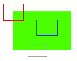
Extracting Certain Objects by Color

To achieve this, we always use the HSV color mode. In HSV mode, it is easier to know the range of a certain color because we only need to modify the range of Hue.

Get the HSV values of blue:

blue = np.uint8([[[255,0,0]]])
hsv_blue = cv.cvtColor(blue,cv.COLOR_BRG2HSV)
print(hsv_blue)

After doing this, we can extract a color from a picture by several steps:

Convert the picture from BGR to HSV
Threshold the HSV picture for a range of the color
Extract objects

Here, we use two functions cv.inRange() and cv.bitwise_and().

cv.inRange(image_input,lower_boundary,upper_boundary) can check if every element in image_input lies in the range. It will set the element to be 255 if it is and set it to be 0 if not. As we only modify the value of Hue to get the range, the output of cv.inRange() should be a black-white picture.
cv.bitwise_and() perform an algorithm that get the product of each element of two images bit-wisely.

Example for Extracting Certain Objects by Color

Source

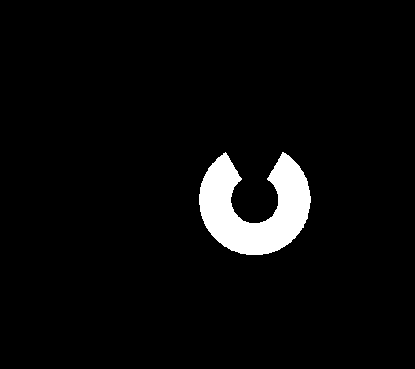
Mask

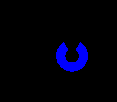
Result

Geometric Transformations

Overview

Transformation basically consists of three operations which are scaling, translation and rotation. As images in OpenCV are stored as matrices that contain the positions of pixels and the channel information. We can simply use the matrix computation to transform images.

Here is a rough idea of how to perform transformation on images.

Generally, the position of a pixel in an image is:

The transformations used for different situations can be described as:

Performing an algorithm below, we can get the new position of the pixel.

By performing the same process on each pixel, we can transform the whole image.

Scaling

Scaling is the operation that resizes the image. In OpenCV, we use the function cv.resize(img,None,sx,sy,interpolation) to complete it.

img: source image
sx, sy: scale along X-axis and Y-axis
interpolation: interpolation method (will be explained after)
The transformation matrix here is:

Using the algorithm, we can easily get new positions of pixels either in a bigger image or a smaller one. However, the number of pixelx is fixed, so we need interpolation to either fill the vacancies or condense pixels. Different methods are used here.

cv.INTER_AREA: for shrinking
cv.INTER_CUBIC: for zooming but is slow
cv.INTER_LINEAR: for zooming and is the default method

Scaling an image example

Source

Scaled

Translation

Translation is actually moving every pixel in the image. In OpenCV, we use displacements along X-axis and Y-axis to complete this process.

The transformation matrix here is:

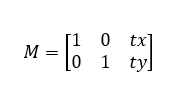
The function we used here is cv.warpAffine(img,M,area) which contains three arguments.

img: source image
M: the transformation matrix
area: the display area of new image with the form of (width, height)

Having this function, we can pass the matrix to it once we know the displacements.

Example for Translation

Source

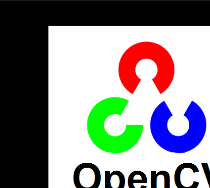
Translated

Rotation

Rotation of an image can also be achieved by matrix algorithm.

When rotating with the original center, the transformation matrix is:

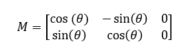
When rotating with adjustable center, the process can be seperated into three steps:

translate from original point to rotation center
rotate with center
translate backward

In OpenCV, we can use cv.getRotationMatrix2D() to get the rotation matrix with adjustable center. The three arguments in function cv.getRotationMatrix2D() are rotation center(given in brackets), angle and scale which means that the matrix also contains the function of scaling. Once we get the rotation matrix, we can pass it to function cv.warpAffine() to complete rotation.

Example for Rotation

Source

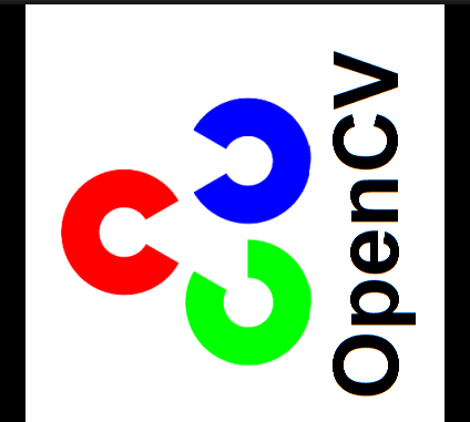
Rotated

CONTOURS AND HISTOGRAMS

Contours

In OpenCV, contours can be seen as curves that connect all the continuous points along the boundary with the same color and intensity. Here, I will simply introduce contours.

Finding contours

To achieve finding contours, we use the function cv.findContours(img,mode,method)

img: source image
mode: contour retrieval mode
method: contour approximation method

This function is like finding a white object in a black background. It will perform better if use the funciton cv.threshold() to convert image to a binary image.

The output contours is actually a list of points. The hierarchy is affected by the contour retrieval mode and represents the ranks of contours. Generally speaking, it represents the parent-child relationship where external contours are parents. For more details of hierarchy, check the link here.

For the approximation methods, there are two commonly used methods:
cv.CHAIN_APPROX_NONE: returns all points
cv.CHAIN_APPROX_SIMPLE: returns less points

If the shape of contour is not very complex, using cv.CHIAN_APPROX_SIMPLE can save time effectively.

Drawing contours

Use cv.drawContours(img,contours,index,(color),thickness):

img: source image
contours: the list of contour points
index: index of contour(use -1 to draw all contours or other number to draw certain contour)
color: color in BGR mode
thickness: thickness of contours

Contours example

All contours

Certain contour

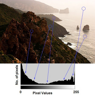
Histogram

Histogram is a plot which shows the intensity distribution of an image. The pixel value is on X-axis and number of pixels is on Y-axis.

Here is an example of histogram from official website

In OpenCV, we use the function cv.calcHist(image,[channels],mask,histSize,ranges)

image: source image
channels: index of channel for calculating histogram(given in square brackets)
mask: mask image used to restrict the area to calculate(None for full area)
histSize: the size of bin(seperate the whole value interval into subintervals with same size)
ranges: the value range to calculate(normally [0,256])

Example: Calculate histogram in OpenCV

Source

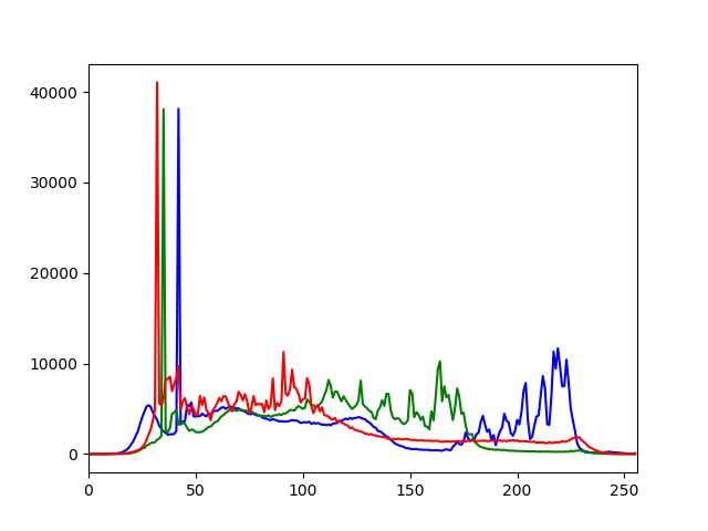
Histogram

EXTRA EXAMPLES - Feature detection, description and matching

There are a bunch of algorithms incorporated in OpenCV to perform feature detection. As this workshop has a finite time we wanted to introduce you all to a couple of them. In case you are interested in you can have a look to the main page to get a deeper sense for all of them.

We have though that will be interesting to have a look to a corner detection and tracking objects.

Basics on corner detection

The basic idea of corner detection falls in moving a patch all over the image. Hence, detecting for example a bit of the interior of a green square is difficult because all of it is green and uniform. Secondly, imagine one of the sides is desired to be detected. This is going to be easier to detect but difficult to locate the exact position. Finally, find out a single corner is easy because wherever the patch is analyzing the image it will look different.

Harris corner detection is one of the simplest algorithms to do feature detection. There are many more refined algorithms to improve the results. Check the following link for further details of the provided algorithms by OpenCV. Feature detection algorithms.

Video analysis

Tracking with meanshift and camshift

Before this chapter we will have already presented the color tracking (changing colorspaces tab), but now the algorithm will be able to track the feature through all the video frames.

The simple idea falls into defining a target to be followed, this image is transformed into a backprojected histogram (like filtering the target and deleting the rest) where the high density of points turns out into our target. Due to the movement of the target the high density of points is also moved. At this point, the algorithm looks for again the high-density region moving the pre-defined window. This process is repeated over and over till the window finds the maximum density region of points.

The idea of both algorithms is the same the only difference is that Camshift calculates the orientation of the target and resizes the window identifying it. Camshift is considerated an upgraded version of the Meanshift.

For further information and examples visit OpenCV guide for meanshift and camshift

Computational Modelling Tools Workshops

Introduction to OpenCV

Getting started with the VM

OpenCV - Python Installation

Workshop material

Pulling last version of the repository examples

OpenCV

Getting started with OpenCV

Managing Images

Managing Videos

Basic image and video manipulations

Changing Colors Spaces

Geometric Transformations

CONTOURS AND HISTOGRAMS

Contours

Histogram

EXTRA EXAMPLES - Feature detection, description and matching

Video analysis

Getting started with the VM

OpenCV - Python Installation

Workshop material

Pulling last version of the repository examples

OpenCV

Getting started with OpenCV

Managing Images

Managing Videos

Basic image and video manipulations

Changing Colors Spaces

Geometric Transformations

CONTOURS AND HISTOGRAMS

Contours

Histogram

EXTRA EXAMPLES - Feature detection, description and matching

Video analysis

blogroll

social